DryVR’s Verification Language¶

In DryVR, a hybrid system is modeled as a combination of a white-box that specifies the mode switches (Transition Graph) and a black-box that can simulate the continuous evolution in each mode (Black-box Simulator).

Black-box Simulator¶

The black-box simulator for a (deterministic) takes as input a mode label, an initial state $x_0$ , and a finite sequence of time points $t_1, \ldots, t_k$ , and returns a sequence of states $sim(mode,x_0,t_1), \ldots, sim(mode,x_0,t_k)$ as the simulation trajectory of the system in the given mode starting from $x_0$ at the time points $t_1, \ldots, t_k$ .

DryVR uses the black-box simulator by calling the simulation function:

TC_Simulate(Modes,initialCondition,time_bound)

Given the mode name “Mode”, initial state “initialCondition” and time horizon “time_bound”, the function TC_Simulate should return an python array of the form:

[[t_0,variable_1(t_0),variable_2(t_0),...],[t_1,variable_1(t_1),variable_2(t_1),...],...]

We provide several example simulation functions and you have to write your own if you want to verify systems that use other black-boxes. Once you create the TC_Simulate function and corresponding input file, you can run DryVR to check the safety of your system. To connect DryVR with your own black-box simulator, please refer to section Advanced Tricks: Verify your own black-box system for more details.

Transition Graph¶

The transition of Automatic Emergency Braking (AEB) system

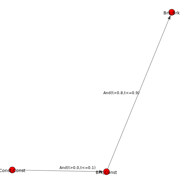
A transition graph is a labeled, directed graph as shown on the right. The vertex labels (red nodes in the graph) specify the modes of the system, and the edge labels specify the guard and reset from the predecessor node to the successor node.

The transition graph shown on the right defines an automatic emergency braking system. Car1 is driving ahead of Car2 on a straight lane. Initially, both car1 and car2 are in the constant speed mode (Const;Const). Within a short amount of time ([0,0.1]s) Car1 transits into brake mode while Car2 remains in the cruise mode (Brk;Const). After [0.8,0.9]s, Car2 will react by braking as well so both cars are in the brake mode (Brk;Brk).

The transition graph will be generated automatically by DryVR and stored in the tool’s root directory as curGraph.png

Input Format¶

The input for DryVR is of the form

{
  "vertex":[transition graph vertex labels (modes)]
  "edge":[transition graph edges, (i,j) means there is a directed edge from vertex i to vertex j]
  "variables":[the name of variables in the system]
  "guards":[transition graph edge labels (transition condition)]
  "resets":[reset condition after transition] # This is optional if you do not want reset
  "initialVertex":integer indicates the vertex to start # This is optional for DAG graph
  "initialSet":[two arrays defining the lower and upper bound of each variable]
  "unsafeSet":@[mode name]:[unsafe region]
  "timeHorizon":[Time bound for the verification]
  "directory": directory of the folder which contains the simulator for black-box system
  "bloatingMethod": specify the bloating method, which can be either "PW" or "GLOBAL" # This is optional, if you don't have this field in input file, DryVR will use GLOBAL as default bloating method.
  "kvalue": specify the k-value that used by piecewise bloating method # This field must be specified if you choose the bloatingMethod to "PW"
}

Some fields are optional in DryVR’s input langauge such as resets, initialVertex, bloatingMethod and kvalue under some conditions. Please read the comment.

Example input for the Automatic Emergency Braking System

{
  "vertex":["Const;Const","Brk;Const","Brk;Brk"],
  "edge":[[0,1],[1,2]],
  "variables":["car1_x","car1_y","car1_vx","car1_vy","car2_x","car2_y","car2_vx","car2_vy"],
  "guards":[
    "And(t>0.0,t<=0.1)",
    "And(t>0.8,t<=0.9)"
  ],
  "initialSet":[[0.0,0.5,0.0,1.0,0.0,-17.0,0.0,1.0],[0.0,1.0,0.0,1.0,0.0,-15.0,0.0,1.0]],
  "unsafeSet":"@Allmode:And(car1_y-car2_y<3, car2_y-car1_y<3)",
  "timeHorizon":5.0,
  "directory":"examples/cars"
}

Output Interpretation¶

The tool will print background information like the current mode, transition time, initial set and discrepancy function information on the run. The final result about safe/unsafe will be printed at the bottom.

The whole verification algorithm will start from doing a few simulations to quickly find the counter-example. If the simulations are all safe, then the main verification process will start. The number of initial simulation can be changed by the user (See {Parameters configuration})

When the system is safe, the final result will look like

System is Safe!

If the verification result is safe, the cooresponding reachtubes are stored in “output/reachtube.txt”

When the system is unsafe from the initial simulations, the final result will look like

Current simulation is not safe. Program halt

When the system is unsafe from the verification process, the final result will look like

System is not safe in Mode [Mode name]

When the system is unknown from verification, the final result will look like

Hit refine threshold, system halt, result unknown

If the simulation result is not safe from the initial simulations, the unsafe simulation trajectory will be stored in “output/Traj.txt”.

If the verfication result is not safe from the verification process, the counter example reachtube will be stored in “output/unsafeTube.txt”.

Advanced Tricks: Verify your own black-box system¶

We use a very simple example of a thermostat as the starting point to show how to use DryVR to verify your own black-box system.

The thermostat is a one-dimensional linear hybrid system with two modes “On” and “Off”. The only state variable is the temperature $x$ . In the “On” mode, the system dynamic is

$\dot{x} = 0.1 x,$

and in the “Off” mode, the system dynamic is

$\dot{x} = -0.1 x,$

As for DryVR, of course, all the information about dynamics is hidden. Instead, you need to provide the simulator function TC_Simulate as discussed in Black-box Simulator.

Step 1: Create a folder in the DryVR root directory for your new model and enter it.

cd examples
mkdir Thermostats
cd Thermostats

Step 2: Inside your model folder, create a python script for your model.

touch Thermostats_ODE.py

Step 3: Write the TC_Simulate function in the python file Thermostats_ODE.py.

For the thermostat system, one simulator function could be:

def thermo_dynamic(y,t,rate):
    dydt = rate*y
    return dydt

def TC_Simulate(Mode,initialCondition,time_bound):
    time_step = 0.05;
    time_bound = float(time_bound)
    initial = [float(tmp)  for tmp in initialCondition]
    number_points = int(np.ceil(time_bound/time_step))
    t = [i*time_step for i in range(0,number_points)]
    if t[-1] != time_step:
        t.append(time_bound)

    y_initial = initial[0]

    if Mode == 'On':
        rate = 0.1
    elif Mode == 'Off':
        rate = -0.1
    else:
        print('Wrong Mode name!')
    sol = odeint(thermo_dynamic,y_initial,t,args=(rate,),hmax = time_step)

    # Construct the final output
    trace = []
    for j in range(len(t)):
        tmp = []
        tmp.append(t[j])
        tmp.append(sol[j,0])
        trace.append(tmp)
    return trace

In this example, we use odeint simulator from Scipy, but you use any programming language as long as the TC_Simulate function follows the input-output requirement:

TC_Simulate(Mode,initialCondition,time_bound)
Input:
    Mode (string) -- a string indicates the model you want to simulate. Ex. "On"
    initialCondition (list of float) -- a list contains the initial condition. Ex. "[32.0]"
    time_bound (float) -- a float indicates the time horizon for simulation. EX. '10.0'
Output:
    Trace (list of list of float) -- a list of lists contain the trace from a simulation.
    Each index represents the simulation for certain time step.Represents as [time, v1, v2, ........].
    Ex. "[[0.0,32.0],[0.1,32.1],[0.2,32.2]........[10.0,34.3]]"

Step 4: Inside your model folder, create a Python initiate script.

touch __init__.py

Inside your initiate script, import file with function TC_Simulate.

from Thermostats_ODE import *

Step 5: Go to inputFile folder and create an input file for your new model using the format discussed in Input Format.

Create a transition graph specifying the mode transitions. For example, we want the temperature to start within the range $[75,76]$ in the “On” mode. After $[1,1.1]$ second, it transits to the “Off” mode, and transits back to the “On” mode after another $[1,1.1]$ seconds. For bounded time $3.5s$ , we want to check whether the temperature is above $90$ .

The input file can be written as:

{
  "vertex":["On","Off","On"],
  "edge":[[0,1],[1,2]],
  "variables":["temp"],
  "guards":["And(t>1.0,t<=1.1)","And(t>1.0,t<=1.1)"],
  "initialSet":[[75.0],[76.0]],
  "unsafeSet":"@Allmode:temp>91",
  "timeHorizon":3.5,
  "directory":"examples/Thermostats"
}

Save the input file in the folder input/daginput and name it as input_thermo.json.

Step6: Run the verification algorithm using the command:

python main.py input/daginput/input_thermo.json

The system has been checked to be safe with the output:

System is Safe!

We can plot the reachtube using the command:

python plotter.py

And the reachtube for the temperature is shown as

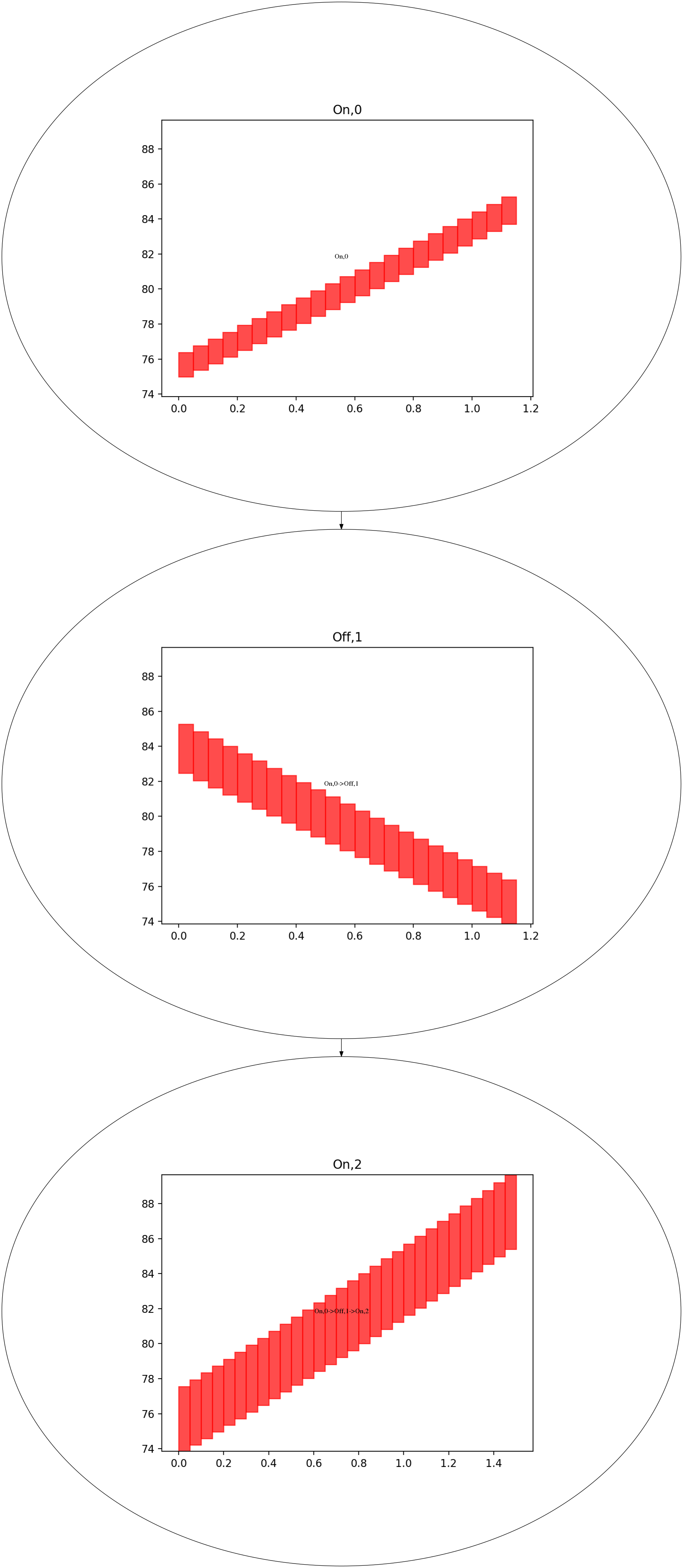
The reachtube for the temperature of the thermostat system example