Examples and Performance Evaluation
Getting started: Simple Automatic Emergency Braking
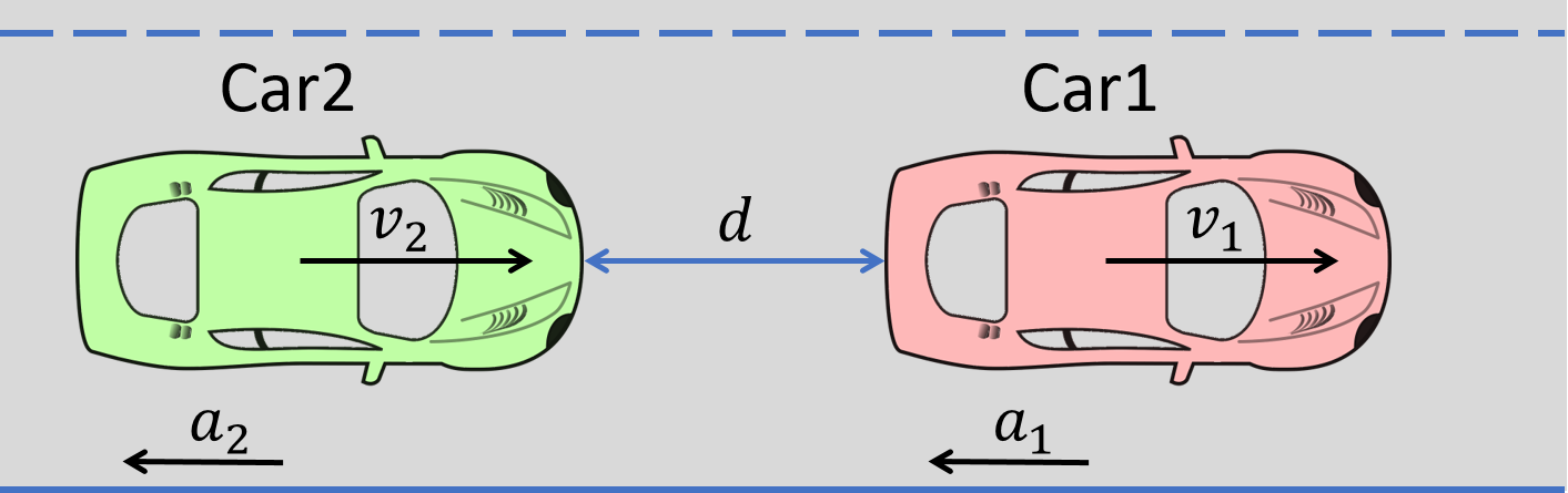
An illustration of Automatic Emergency Braking System
Consider the example an AEB as shown above: Cars 1 and 2 are cruising down the highway with zero relative velocity and certain initial relative separation; Car 1 suddenly switches to a braking mode and starts slowing down according, certain amount of time elapses, before Car 2 switches to a braking mode. We are interested to analyze the severity (relative velocity) of any possible collisions.
Safety Verification of the AEB System
The black-box of the vehicle dynamics is described in The Autonomous Vehicle Benchmark, and the transition graph of the above AEB is shown in Transition Graph. The unsafe region is that the relative distance between the two cars are too close (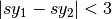 ). The input files describing the hybrid system is shown in Input Format.
Verification Result of the AEB System
Run DryVR’s verification algorithm for the AEB system:
python main.py input/daginput/input_brake.json
The system is checked to be safe. We can also plot the reachtubes for different variables. For example, the reachtubes for the position of Car1 and Car2 along the road the direction are shown below. From the reachtube we can also clearly see that the relative distance between the two cars are never too small.
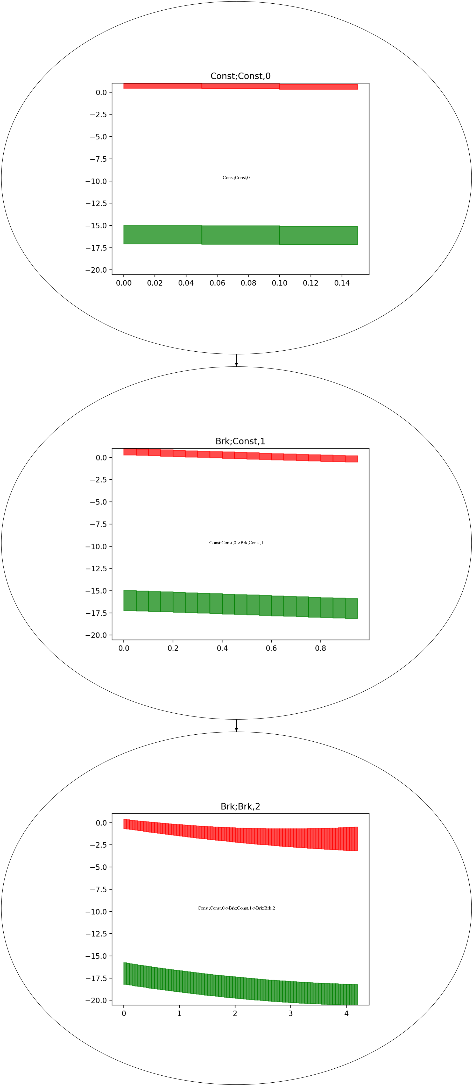
Reachtube of the position sy of Car1 and Car2
The Autonomous Vehicle Benchmark
The hybrid system for a scenario is constructed by putting together several individual vehicles. The higher-level decisions (paths) followed by the vehicles are captured by the transition graphs discussed in Transition Graph.
Each vehicle has the following modes
- Const: move forward at constant speed,
- Acc1: constant acceleration,
- Brk or Dec: constant (slow) deceleration,
- TurnLeft and TurnRight: the acceleration and steering are controlled in such a manner that the vehicle switches to its left (resp. right) lane in a certain amount of time.
The mode for the entire system consists of n vehicles are the mode of each vehicle separated by semicolon. For example, Const;Brk means the first car is in the const speed mode, while the second car is in the brake mode.
For each vehicle, we mainly analyze four variables: absolute position
( ) and velocity (
 ) orthogonal to the road direction
(
) orthogonal to the road direction
( -axis), and absolute position (
 ) and velocity (
 ) along the
road direction (
) along the
road direction ( -axis). The throttle and steering is captured using the four variables.
Verification Examples
DryVR now comes with more than two dozen interesting examples, including
- 6 mixed-signal circuit models with hundreds of nonlinear terms in the dynamics and both time and state dependent transitions
- 6 high dimensional linear system models (up to 384 dimensions)derived from fields such as civil engineering and robotics
- an 8-dimensional hybrid vehicle lane switch model modeling a vehicle switches its lane on highway if it get too close to another vehicle in front of it
- a set of standard 2-7 dimensional benchmarks
The simulators for these models are also available in the folder “examples” under the root directory, and the input files are in the folder “input/daginput” and “input/nondaginput”.
Verification Peformance Evaluation
We have measured performance for examples come with DryVR 2.0. Peformance is measured using computer with i7 6600u, 16gb ram, Ubuntu 16.04 OS.
| Model | Dimension | Time for 1 simulation | Total Time | Flow* time |
| Biological model I | 7 | 0.01s | 0.04s | 66.4s |
| Biological model II | 7 | 0.01s | 0.04s | 223.4s |
| Coupled Vanderpol | 4 | 0.03s | 0.14s | 1038.3s |
| Spring pendulum | 4 | 0.05s | 0.16s | 1377.5s |
| Roessler | 3 | 0.02s | 0.36s | 17.1s |
| Lorentz system | 3 | 0.34s | 1.07s | 316.7s |
| Lac operon | 2 | 0.47s | 171.35s | 44.2s |
| Lotka-Volterra | 2 | 0.02s | 0.10s | 3.9s |
| Buckling column | 2 | 0.04s | 0.43s | 26.4s |
| Jet engine | 2 | 0.07s | 12.1s | 6.8s |
| Brusselator | 2 | 0.10s | 3.02s | 5.2s |
| Vanderpol | 2 | 0.05s | 2.92s | 6.4s |
| Vehicle platoon 3 | 9 | 0.32s | 4.28s | 21.08s |
| Uniform nor sigmoid | 3 | 120.91s | 1314.22s | Exception |
| Uniform inverter loop | 2 | 10.94s | 278.56s | Exception |
| Uniform inverter sigmoid | 2 | 24.87s | 246.76s | Exception |
| Uniform nor ramp | 3 | 173.77s | 1765.55s | Exception |
| Uniform or ramp | 4 | 176.70s | 1778.87s | Exception |
| Uniform or sigmoid | 4 | 168.75s | 2186.00s | Exception |
| Clamped beam | 348 | 540.80s | 5717.63s | Time out |
| Building model | 48 | 3.28s | 20.24s | Time out |
| Partial differential equation | 20 | 12.05s | 41.21s | Time out |
| FOM | 20 | 12.18s | 40.9s | Time out |
| Motor control system | 8 | 5.22s | 17.89s | Time out |
| International space station | 25 | 79.99s | 243.60s | Time out |
| Lane switch | 8 | 0.29s | 563.52s | N/A |
Synthesis Examples
We provide 6 controller synthesis benchmarks examples, including:
- A vehicle collision avoidance model where a car driving on the highway is asked to avoid an obstacle in front of it.
- Robot find a path in a maze.
- Motion planning from synthesis tool Pessoa with specification similar to Example 2.
- DC motor where the velocity of a DC motor needs to be regulated.
- Room heating where the task is to control the temperature of 3 rooms and keep them around 21.
- Inverted pendulum as a classical reach-avoid problem.
Synthesis Performance Evaluation
Peformance is measured using computer with i7 6600u, 16gb ram, Ubuntu 16.04 OS. Note the running time for graph search can be very different since the alogirthm is randomly search for the graph. It may also return nothing as well. Try to run algorithm multiple times if it does not return the graph.
| Example | Dimension | Time horizon | Min staying time | Running Time |
| vehicle collision avoidance | 4 | 50.0s | 2.0s | 1896.26s |
| robot in maze | 4 | 10.0s | 1.0s | 98.93s |
| motion plan | 3 | 6.0s | 1.0s | 4.55s |
| DC motor | 2 | 1.0s | 0.1s | 0.35s |
| room heating | 3 | 25.0s | 2.0s | 2.66s |
| inverted pendulum | 2 | 2.0s | 0.2s | 6.06s |